Studying Neural Cell Types to Understand Neural Function
To understand the brain, we must understand neurons, the brain's 'logic gates'. In this piece, I tentatively define 'neural function' and reflect on how neural "cell-typing" can help us understand neural function.
Biologists have classified neurons into cell-types for decades. While early anatomists relied exclusively on anatomy and morphology to define neuron types, modern techniques now provide us with tremendously more information to profile neurons, including their molecular and electrophysiological characteristics. In this piece, I explore the key motivations that drove earlier biologists—and continue to drive us—to study neuron cell-types, such as in our recent paper published last week in Cell (Beau et al., 2025).
I am very proud to announce that my PhD paper finally came out in Cell! In this *very* collaborative study, we develop and release a deep-learning approach to predict neuron type identity from their electrical signature. doi.org/10.1016/j.ce... 1/16 🧵
— Maxime Beau (@maxime-beau.bsky.social) 1 March 2025 at 13:14
[image or embed]
Neuron cell-typing has pretty broad implications for neuroscience:
- It supports reproducibility in neuroscience by establishing shared nomenclatures that create a common language, making results comparable and allowing research efforts to work in synergy.
- It enables molecular targeting of specific neurons, with numerous applications both in physiology and pathology. For example, it allows us to read and write neural activity by expressing calcium sensors and opsins in precisely targeted neuron populations.
- It is critical for studies in evolution and development, providing a foundation for comparative anatomy at the cellular level and for understanding cellular fate determination.
- Finally, a comprehensive neural cell-types nomenclature would facilitate the quest to understand neural function by shifting from billions of individual neurons to hundreds of cell-type groups, under the assumption that neurons sharing the same cell-type also share specialized computational roles.
Below, I develop this last point across four sections. First, I establish a clear definition of ‘neural function’ and related epistemological terms. Then, I examine which neuron features correlate with neural function. Third, I explain how neural cell-types can be formally defined based on these neural features. Finally, I present example from specific brain regions where neural cell types have been shown to map closely onto neural function.
What do we mean by ‘neural function’?
Biology can be defined as the quest to understand the function of cells, organs, and organisms. Neuroscience, then, is the quest to understand the function of neurons, circuits, and neural systems. Neuroscientists refer to ‘neural function’ all the time, and below is my clumsy attempt at defining this term. I also use this opportunity to define frequently employed epistemological terms for my mental sanity, such as ‘correlation’, ‘causality’, the distinction between ‘bug’ versus ‘feature’, or ‘emergent properties’.
‘Function’ is defined as “the purpose (of something) or the duty (of a person) within a larger context”. The concept of context here is critical here. Indeed, a function can only be defined with respect to a larger system of reference (e.g. a protein w/r a cell, a cell w/r an organ, an organ w/r an organism). The ‘function’ of smaller components can then be studied in relation to this reference. A discussion that often arises when discussing the concept of ‘function’ is the question of intelligent design, as ‘function’ in layman’s terms refers to an ‘intended purpose’. Intended by what, or whom? In modern biology, the ‘function’ of structures is of course not meant in the teleological sense, where organisms would be the result of intelligent or religious design. Function is meant in the teleonomical sense — an apparent purposefulness arising from natural processes such as evolutionary pressures.
In practice, biologists cannot directly estimate the function of a structure, because biological objects are discovered, not engineered. Biologists can only measure statistical relationships between variables observed in nature. This practice relies on: 1) choosing a structure (variable) of reference, 2) reporting statistical dependency between other biological variables and this reference (which can be quantitative, e.g. the firing rate of a neuron and behaviour, or qualitative, e.g. the presence of a phosphorylated protein and cell survival). While we colloquially use the term ‘correlations’ to report any form of statistical dependence, this term formally refers exclusively to linear dependence (Figure 1, A). After observing that two variables are statistically dependent in observational studies, we design interventional studies to reveal necessity or sufficiency relationships. Note that ‘causal’ relationships are equivalent to ‘sufficiency’ relationships. If neither necessity nor sufficiency is found, the statistical dependence between the variables is considered spurious. Spurious dependence (or correlation) occurs when a third hidden variable (‘h’ in Figure 1, A) causes two variables to exhibit statistical dependence. This hidden variable is called a ‘confound’, and may result from the method used to select samples (selection bias, e.g. the infamous survivor bias) or from a hidden, latent process influencing both variables (e.g. Simpson’s paradox). In summary, biologists aim to estimate whether sub-structures have functions with respect to a larger structure of reference, by identifying candidate necessity and/or sufficiency relationships between these structures through observational studies and testing these relationships through interventional studies.
💡 Note
Here, sufficiency (causality) and necessity refer to relationships between structures across scales. Commonly, sufficiency and necessity refer to relationships between events across time. I do not discuss the conceptual differences between relationships between structures across scale or events across time, but this distinction is intriguing and deserves further discussion.
This definition of ‘function’ allows us to precisely define related epistemological terms (Figure 1, B). As mentioned above, we can concisely define function in biology as the teleonomical purpose of a substructure in relation to a larger structure, formally captured by necessity and/or sufficiency relationships. The connection between discovering ‘function’ and necessity/sufficiency relationships is also apparent is the naming of interventional studies. Loss of function experiments reveal necessity relationships, while gain of function experiments reveal sufficiency relationships. A feature refers to a substructure that is either necessary or sufficient for the existence of a larger structure’s property. It is a characteristic likely selected for or maintained through evolutionary processes due to its beneficial effects. In contrast, a bug is a subtructure that might be truly (non-spuriously) correlated with a larger structure but whose presence or absence has no effect on it (E.g. genetic drift, or vestigial anatomical structures). In summary, when a substructure is necessary or sufficient for the proper operation of a larger system, it is a feature of this system, and the specifics of how it contributes to this system define the substructure’s function.
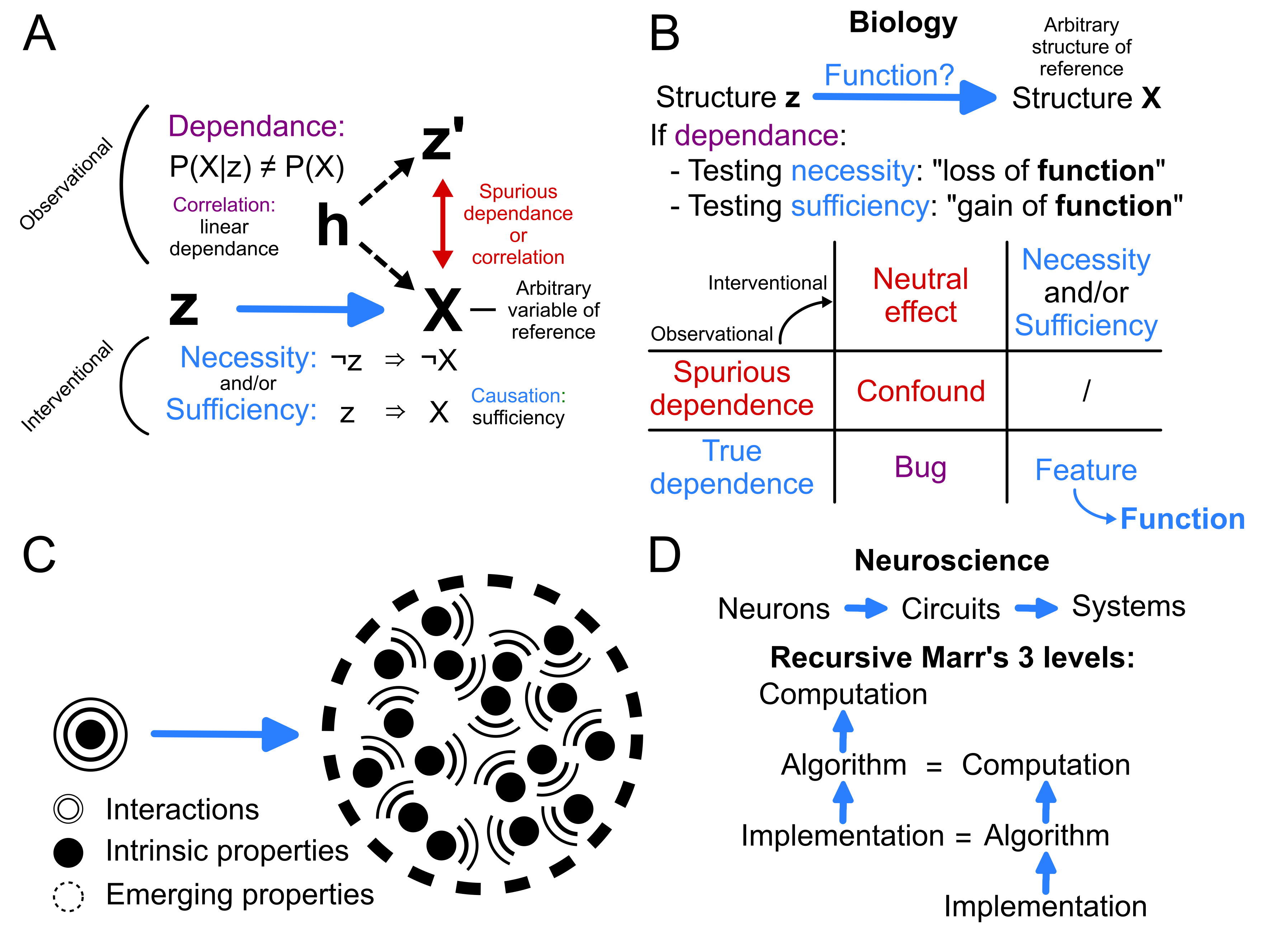
A. In practice, biologists cannot directly determine whether a structure has a function, as biological objects are discovered, not engineered. Biologists can only measure statistical relationships between variables in nature. This requires arbitrarily defining a reference variable \(X\): once established, all other variables \(z\) are evaluated in relation to it. Observational studies measure dependence with respect to the reference (\(P(X|z) \neq P(X)\)). When dependence is found, it may reveal a relationship of necessity or sufficiency. The common colloquial terms correlation and causation correspond to relationships of linear dependence and sufficiency, respectively. Statistical dependence between variables can also be spurious, when a hidden latent variable \(h\), a confound, correlates with both the variable under study and the reference. In this figure, thick blue arrows denote relationships of necessity or sufficiency, while thin red double arrows denote relationships of spurious dependence.
B. If an observational study reveals a true dependence between the presence of a sub-structure and a property of a larger structure of reference, interventional studies can employ loss or gain of function experiments to determine whether the substructure is necessary or sufficient for the existence of the larger structure's property. A feature refers to a substructure that is either necessary or sufficient to the existence of a larger structure's property (likely selected through evolutionary processes). In contrast, a bug is a substructure that might truly correlate with a larger structure but whose presence or absence has no effect on the larger structure. In summary, when a substructure is necessary or sufficient for the proper operation of a larger system, it is a feature of this system. How it contributes to this system defines its function.
C. When examining the function of small structures with respect to larger reference structures, describing the function of the small structures alone may be insufficient to capture the properties of the reference structure. This occurs because the whole can exceed the sum of its parts: some properties of complex systems are emergent, i.e. they are a byproduct of the interactions between their constituents but do not exist within them intrinsically. Thus, a complete description of a component's function within a larger biological system should address both the system properties directly related to intrinsic properties of the underlying components, and those that emerge from interactions between these components.
D. While the structure/function typology predominates in biology, Marr's three levels do in neuroscience. The computational level defines the goal of the computing system, its 'objective function'. The algorithmic level defines the strategy(ies) to reach that goal. The implementation level defines the physical substrate that implements these algorithms. Marr's three levels provide a valuable framework for studying computing systems. Drawing from Dean & Porrill (2016), I define the `recursive Marr's 3 levels', which explicitly extends them to relative scales of analysis within a deep hierarchical computing system. They proved useful to define two scales of Marrian `computational' level at two scales in my PhD thesis introduction of cerebellar structure and function: the intrinsic computations operated by the cerebellar microcomplexes in the cerebellum, and the extrinsic computations operated by the cerebellum in the brain.
We mentioned that the function of a component can only be defined within a larger context - that is, with respect to a larger system of reference. When considering the function of small structures with respect to larger reference structures, it’s important to recognize that describing the constituents of complex systems often doesn’t fully capture them - the whole can be greater than the sum of its parts. This occurs because some properties of complex systems are ‘emergent’, arising as byproduct of interactions between their constituents rather than existing within them individually (Figure 1, C). Much as describing a bird in a flock requires describing not only its structure and directly derived properties (wings that enable flight) but also its interactions with other birds (maintaining set distances) to explain the emergence of chaotic patterns in murmurations. Thus, a complete functional description of a component within a larger biological system should include both intrinsic properties of the underlying components and emergent properties in the larger system resulting from interactions between the components. For instance, the capacitance of a neural membrane simply amounts to the linear sum of the capacitance of small patches of this membrane. However, the conductance of a neural membrane results from many complex non-linear interactions between various kinds of ion channels, trans-membrane voltage, and neurotransmitters. Importantly, note that necessity or sufficiency relationships can exist between objects of comparable complexity, in which case choosing a structure of reference becomes arbitrary. Consider the symbiotic relationships between algae and corals, or the interdependence between the pulmonary and cardiovascular systems.
To define what we mean by ‘neural function’, I have revisited the traditional structure/function typology common in biology. In neuroscience, however, this typology is often overshadowed by another: Marr’s 3 levels of analysis. This influential framework, proposed by David Marr for understanding information processing systems, comprises three levels:
- Computational level: This level addresses the “what” and “why” of the system. It defines the goal of the computing system. It focuses on the problem being solved.
- Algorithmic level: dealing with the “how” of the system, this level describes the specific algorithm or procedure used to carry out the computation, including input and output representations.
- Implementation level: This level concerns the physical realization of the system. It describes how the algorithm is actually implemented in hardware, such as neurons in the brain or transistors in a computer.
These levels provide a structured approach to analyzing and understanding complex systems, from their abstract purpose down to their concrete physical implementation. They also directly relate to the structure/function typology: the ‘function’ of the implementation level can be viewed as supporting the algorithmic level, whose ‘function’ can in turn be viewed as supporting the computational level.
Marr’s three levels of analysis provide a robust framework for understanding information processing systems, which I’ve extended them to freely apply them across scales of analysis. Consider a system designed with the objective to sort an array. The computational level, ‘why’, would be ‘sorting’; the algorithmic level, ‘how’, would be strategies such as merge-sort or quick-sort; and the implementation level could be Python code. However, the algorithm ‘quick-sort’ could be chosen as the target computation; in which case, Python or C++ programs would become the algorithmic level, and assembly language the implementation level. Following these reflections and inspired by Dean & Porrill (2016), I coin the term ‘recursive Marr’s three levels’ to explicitly denote their expansion to relative scales of analysis within a deep hierarchical computing system, such as the cerebellum circuit embedded in the brain (Figure 1, D). Specifically, though less relevant for this specific post, I define a Marrian computational level over two scales in my introduction of cerebellar structure and function, analogously to the Dean & Porrill (2016) ‘chip metaphor’: the intrinsic computations operated by the cerebellar microcomplexes in the cerebellum, and the extrinsic computations operated by the cerebellum in the brain.
Neural features correlate with neural function
Several properties of neurons can be directly or indirectly linked to their function. It all starts from the molecular repertoire of neurons and used to define neural cell-types. Their genetic material - DNA, epigenome and RNA - governs the expression of proteins which collectively support all aspects of a neuron’s fate (Figure 2, A, blue boxes). Morphogenes and recognition molecules are responsible for the migration of neurons to their ultimate anatomical location and also guide the formation of synapses with mechanisms guiding partner recognition and self-avoidance. The connectivity between two neurons is also conditional to their anatomical location, an observation which is the premise of Peters’ rule (Figure 2, A, left): “postulated that, if neurons of type A project their axons to brain regions i, j, and k, the existence and amount of their synaptic connections to neurons of type X and Y primarily depend on the dendritic extent of X and Y in those same regions”. The evidence for this simplistic view of the forces driving connectivity has been reevaluated extensively, but everyone agrees on the fact that the formation of at least one synapse between two neurons is conditional to the co-location of their neurites. The morphology of neurons also relies directly on adhesion and recognition molecules as a trail of membranous processes can be left in the path of the migration of their soma during development and because mechanisms such as self-avoidance cause their processes to radiate in space. The morphology of neurons then constrains their connectivity, just like their anatomical location does, since the morphology of neurons guides their co-location with other neurons. Conversely, the connectivity between neurons also influences their morphology, as their membranous processes can be pulled towards their synaptic partners during development (Figure 2, A, green boxes). Lastly, the pool of ion channels distributed across the membranes of neurons and the morphology of neurons influence the generation and propagation of spikes, respectively (Figure 2, A, green box ‘Physiology’). Indeed, a highly ramified dendritic tree prevents action potentials from backpropagating (e.g. in cerebellar Purkinje cells), whereas consistently cylindrical dendrites facilitate backpropagation (e.g. in neocortical pyramidal neurons). Voltage-gated ion channels exhibit distinct biophysical properties and gating kinetics: Nav channels activate rapidly (within <1 ms) in response to membrane depolarization and typically inactivate within 1-2 ms, whereas HCN channels are uniquely activated by hyperpolarization with slower kinetics (tens to hundreds of ms). Ionotropic glutamate receptors also display characteristic temporal profiles: AMPA receptors show rapid activation (~0.2-0.4 ms) and deactivation (~1-2 ms), while NMDA receptors exhibit slower activation (~7-10 ms) and deactivation kinetics (~50-100 ms). Some K+ channels, particularly the two-pore domain (K2P) family, maintain a voltage-independent “leak” conductance that contributes to the resting membrane potential. High-voltage activated L-type Ca2+ channels can sustain prolonged openings during plateau potentials in dendrites, which can trigger somatic burst firing patterns. In fact, the same channel can fulfil different functions (pleiotropy), and different channels can fulfil the same function (degeneracy). This diversity causes neurons with different channel pools to discharge with different intrinsic firing and different waveform temporal profiles.
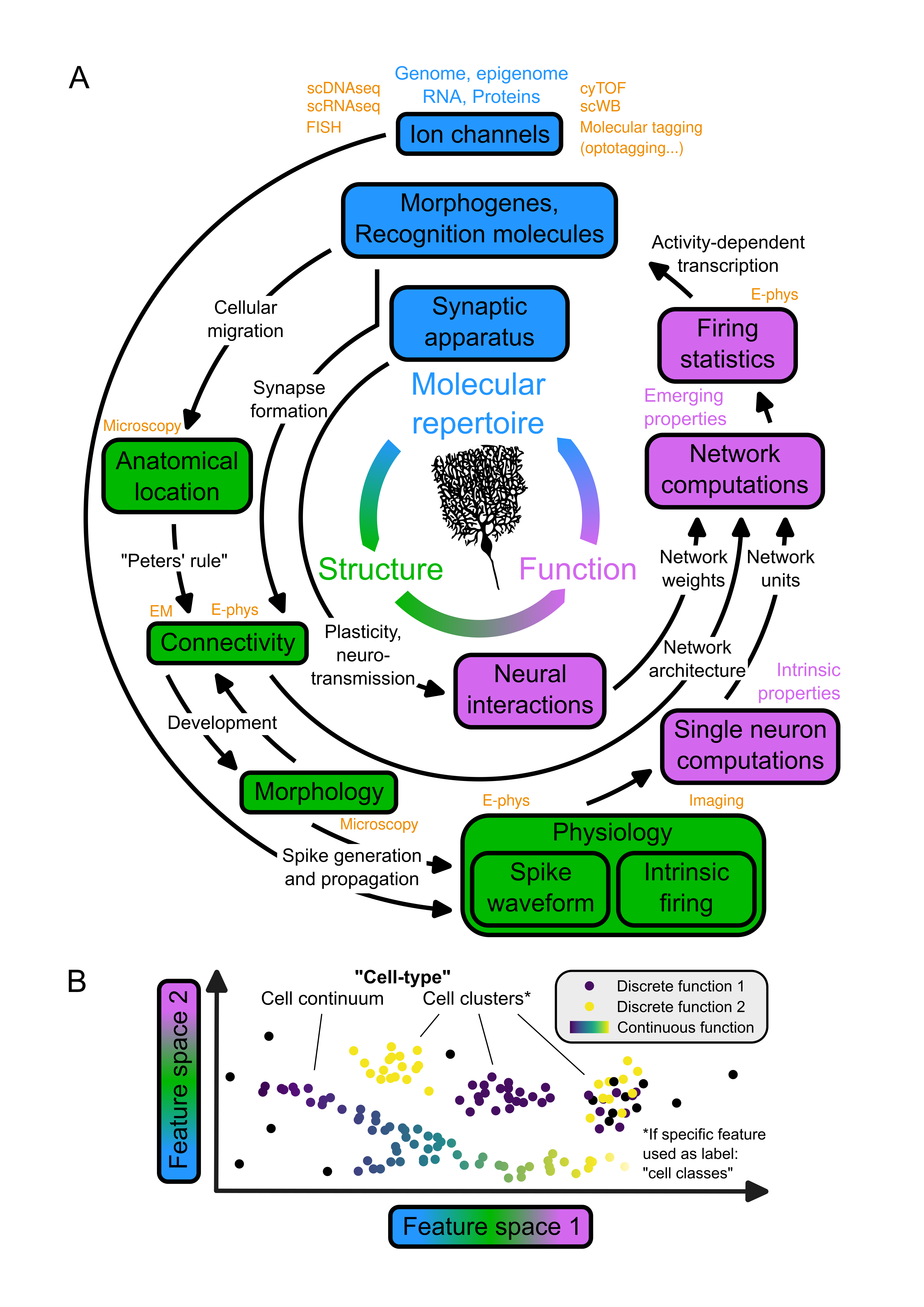
A: Model of the relationship between the molecular repertoire, structure, and function of neurons.
The molecular repertoire of a neuron (blue) plays a dual role in shaping not only the neuron's intrinsic properties but also in governing its connectivity and interactions with other neurons. The computations within a neural network are emerging properties resulting from the interplay between these intrinsic properties and inter-neuronal interactions. Describing Neural function (purple) requires describing both the intrinsic properties of neurons and the emerging properties of neural networks. The pathways linking the molecular repertoire of a neuron to its function involve several actors that can be listed as elements of the structure of neurons (green). Finally, it is important to note that the activity of a neuron has an influence on its molecular repertoire via activity-dependent transcription factors, closing the loop between molecular repertoire, structure and function. Features of single neurons distributed across this loop can be probed with several methods from molecular biology and neuroscience (orange).
B: Definition of neural cell-types and relationship with neural function.
Each datapoint on the scatter plot represents a neuron, and the two axes represent two dimensions derived from the hyperspace of features defined in A (for instance, the spike waveform shape, firing statistics and anatomical location of neurons). These two dimensions could either result from a linear transformation such as principal component analysis (PCA), or from a non-linear transformation such as uniform manifold approximation and projection (UMAP) or the encoding of a variational autoencoder (VAE). In the feature hyperspace, neurons can cluster or lay along a continuum (Harris et al., 2018). These groups of neurons can emerge from the data and be unveiled with models trained with unsupervised learning (clustering). Alternatively, these groups of neurons can be predefined into classes based on labels (e.g. Purkinje cells, defined morphologically) and their class can be predicted from their position in the feature hyperspace with models trained with supervised learning (classification). In Beau et al., 2025, we developed an algorithm for cell type classification of neurons in the cerebellum cortex. The goal of cell-type classification is to group neurons into functionally homogeneous classes, whether they map onto discrete (Kozareva et al., 2021) or continuous (Bugeon et al., 2022) functions.
scDNAseq: single-cell DNA sequencing; scRNAseq: single-cell RNA sequencing; FISH: Fluorescence In Situ Hybridization; cyTOF: flow cytometry by Time Of Flight; scWB: single-cell Western Blot; E-phys: electrophysiology; Imaging: Calcium or voltage imaging; EM: Electronic Microscopy.
Taken together, these properties determine the highly non-linear single neuron computations operated by neurons to transform their inputs into their outputs (Figure 2, A, purple boxes). These transformations can be very complex, ranging from simple linear integration to nonlinear operations equivalent to full-fledged artificial neural networks. It has recently been shown that single human pyramidal neurons could implement the most canonical nonlinear problems: a XOR gate. Using the nomenclature of artificial neural networks as a framework, single neurons can be described as the units of biological networks. In that case, the connectivity of neurons with one another constitutes the architecture of networks, and the synaptic apparatus of neurons (all proteins responsible for neurotransmission and plasticity) are the determinants of network weights. The units, architecture and weights of neural networks constitute the determinants of the computations performed by these networks, which correlate with the firing statistics of the neurons embedded into them (Figure 2, A, purple box ‘Network computations’). Finally, the activity of a network can in turn influence back the molecular repertoire of its neurons, for instance via activity-dependent transcription factors such as c-fos. I would like the reader to note that this perspective on neural function adheres to the conceptual framework unrolled in the previous paragraph, where the function of a neuron is considered in the arbitrary context of “neural network computations” and in relation to a neuron’s intrinsic properties, its interactions between neurons, and the emerging properties of neural networks.
Defining neural cell-types from neural features
Qualitative definition of cell-types
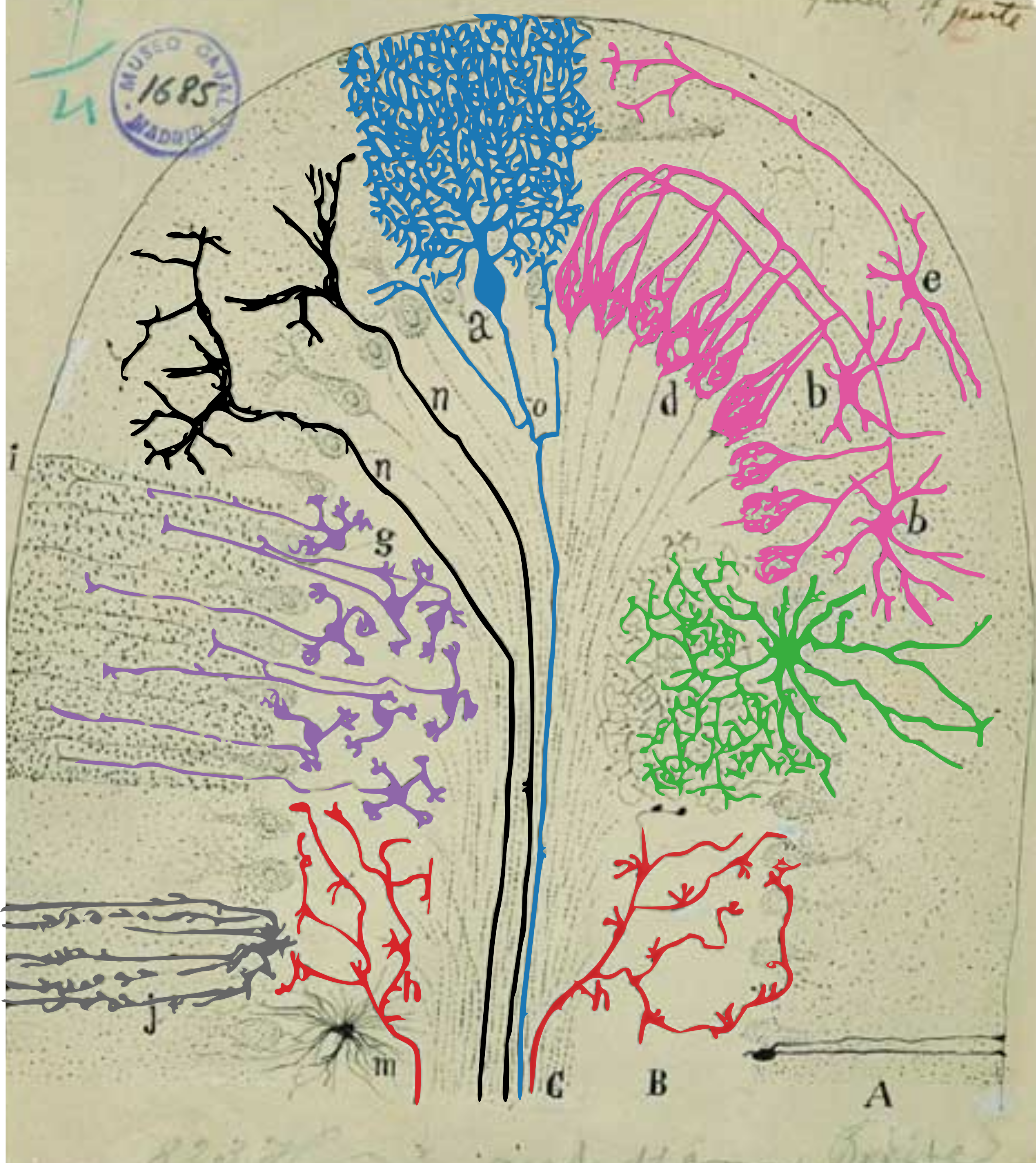
The concept of “Cell types” naturally emerges from the observation that, in all organs, large groups of cells can be grouped into homogeneous “types” that exhibit consistent characteristics. This also stands for neurons. This observation dates from as early as the development of the neuron doctrine with Cajal’s work, which exclusively relied on the anatomical location and morphology of neurons. This explains the original nomenclature of neurons: hippocampal granule cells look like small grains, cerebellar mossy fibres look bushy, neocortical pyramidal cells look like the Louvres’ pyramid (which later inspired the site of Giza). The advent of molecular biology and neuroscience techniques has revolutionized our ability to probe neuronal diversity, far surpassing the capabilities available to early 20th-century neuroanatomists. Modern methods like single-cell DNA sequencing (scDNAseq) and RNA sequencing (scRNAseq) enable the detailed analysis of the genetic and transcriptional landscape of individual neurons. Fluorescent in situ hybridization (FISH) and its derivative, like coppaFISH, can sample joint functional, anatomical and transcriptional information. Cytometry by time-of-flight (CyTOF) and single-cell Western blotting (scWB) extend this molecular characterization to the protein level. Electronic microscopy (EM) allows the exploration of neuronal connectivity and subcellular structures. In addition to these molecular and structural techniques, functional characteristics of neurons are now accessible through calcium or voltage imaging and electrophysiology, which capture the timing and waveform shape of action potentials. Inspirationally, Cajal himself already pointed out that pure reliance on morphological information would never allow us to solve the problem of cell-type classification, as he recognized that the goal of this exercise is to group cells which are ‘dynamically similar’ (we would say, functionally similar):
“This classification, as all others based on purely morphologic principles, is too schematic and artificial. To obtain a more natural grouping of nerve cell types, it is necessary to consider not only the shape and number, but also the structure and length of cell processes. In fact, the shape of the soma, and even the number of processes, varies in neurons of the same type, depending on the distance from the cells with which it relates, and according to certain accommodations ruled by the economy of space and conduction time. In the retina, for instance, the amacrine cells are either unipolar or multipolar, according to the branching pattern of the processes; and in spinal ganglia, the cells are bipolar in fish and unipolar in higher vertebrates. We could cite many other examples that prove the minor importance of the shape of the cell body and its richness in initial processes. They demonstrate that adopting a purely morphologic criterion, could compel us to separate cell types which are dynamically similar, and to group other disparate ones.” Ramón y Cajal, Textura del sistema nervioso del hombre y de los animales (1899–1904)
Machine learning as a formalism to define cell-types
The realization that the goal of cell-type classification is to group functionally similar neurons allows us to loop back to our initial statement: “a comprehensive neural cell-types nomenclature would facilitate the quest to understand neural function”. We showed that this is true because the definition of cell types relies on information, or features, which correlate with neural function. However, because of the plethora of structural and functional features which can be probed with modern techniques, cell-type definition became a dramatically less tractable task than the manual grouping of neuron morphologies achieved by the anatomists of the 20th century. Fortunately, “grouping” or “categorizing” observations in high-dimensional spaces is now well formalized with the statistical framework of machine learning (Figure 2, B). This exercise can be conducted through two primary strategies: unsupervised and supervised learning. These strategies are contingent on the presence or absence of predefined categories (or “labels”) for the neurons under study. In unsupervised learning, employed when neurons do not come with pre-assigned categories (i.e. the neurons are not “labelled”), the ‘grouping’ is based on intrinsic patterns and structures fully inferred from the distribution of neurons in the n-dimensional feature space. This method is referred to as clustering. Many clustering techniques have been developed, such as K-Means, spectral clustering (e.g. DBSCAN) or hierarchical (i.e. agglomerative) clustering. Continua represent a scenario where data points vary substantially within and/or between clusters, which can be assessed with techniques such as negative binomial discriminant analysis (to quantify the overlap between clusters) or latent factor analysis (to attempt to predict neural features from continuous latent variable(s) rather than a discrete distribution of cluster labels) (Harris et al., 2018). On the other hand, supervised learning is applied when neurons are pre-categorized, with each neuron already associated with a specific type based on prior categorization (i.e. the neurons are “labelled”). This method is referred to as classification. Random forest, XGBoost, K-nearest-neighbours, SVM, or multi-layer perceptrons trained with backpropagation on labelled data are example of classification algorithms. A successfully trained classifier learns the hyperplanes separating the classes of the training dataset from each other which can subsequently be utilized for classifying new neurons into these classes. It is important to note that neurons do not necessarily need to spontaneously group into clusters for a hyperplane to exist between predefined neuron classes. Therefore, supervised classification tasks can succeed where unsupervised clustering tasks fail. Imagine a sphere of homogeneously distributed datapoints, where one half is class 1 and the other half is class 2: classes 1 and 2 would not group spontaneously and therefore clustering would fail to identify them, but it is possible to find a plane separating classes 1 and 2. For this reason, it is not because neurons do not spontaneously cluster into groups that it is impossible to train a classifier to distinguish pre-defined cell classes. In Beau et al. (2025), we developed a classifier trained to predict the cell-type of neurons recorded in the cerebellar cortex. In our case, the ‘classes’ of neurons are pre-defined based on the original cell-types defined by Cajal, with the exception of molecular layer interneurons (that were split into stellate and basket cells at the time). The feature space used to predict the neuronal cell-types comprises the anatomical location of neurons, the shape of their extracellular waveform, and their firing statistics summarized as “3D-autocorrelograms”. Refer to the paper for more details.
Example systems where neural cell-types correlate with neural function
I would like to conclude this section with examples of cell-type classification present in the literature, discussing cases where defined cell-types have been successfully associated with particular neural functions and cases where they have not. First of all, the best way to directly test the correspondence between neural features and neural function is to record both simultaneously. Bugeon et al. (2022) have demonstrated how in vivo two-photon calcium imaging of mouse neurons would be used in combination with coppaFISH, a transcriptomic method to identify mRNA for 72 selected genes in ex vivo slices. This method enabled the authors to directly test the correspondence between the molecular repertoire and functional properties of cortical neurons, and found a single transcriptomic axis correlated with the modulation of neurons by the animals’ internal state. This is an example where a continuum of ‘cell-types’ map onto a continuous function (Figure 2). A second interesting example is the history of the classification of cerebellar molecular interneurons. Initially classified into two subtypes, basket and stellate cells, based on their morphology and anatomical location by Cajal, they have been reunified as a single functional group with a gradient of morphologies based on more recent observations. However, recent transcriptomic studies found that there might after all be two sub-classes of molecular layer interneurons, with distinct computational roles. However, these studies found that these two transcriptomic subtypes of interneurons did not correspond to the morphological subtypes defined by Cajal! This example highlights the fact that, because using different neural feature sets can yield different cell-type definitions, neural features should be considered together and treated with the formalism of clustering and classification to define cell types. It also seems like molecular layer interneurons segregate into yet again two categories when clustered based on their action potential waveform shape (Beau et al., 2025, Supplementary Figure 6). A third example is the case of striatal D1 and D2 medium spiny neurons: they are indistinguishable based on their morphology, but express different dopamine receptors (D1 and D2) and project to different brain areas. In this case, transcriptomic studies successfully cluster these neurons into two subcategories which are related to their location in the basal ganglia circuitry, and therefore to their discrete computational role. A fourth remarkable case of successful cell type classification is the case of retinal bipolar neurons. Fifteen classes of bipolar cells (BCs) have been identified from calcium imaging, electron microscopic reconstructions, and single-cell RNA sequencing, and there is little evidence to claim that these neurons belong to a continuum (Figure 3). These 15 clusters can be assembled into three larger functional groups: ON-cone bipolar cells, OFF-cone bipolar cells, and finally rod bipolar cells. The identified transcriptomic relationships parallel the similarities that have been documented morphologically. For example, ON cone bipolar cells are more closely related to each other than they are to OFF cone bipolar cells, and vice versa, and cone bipolar cells are more closely related to each other than they are to rod bipolar cells.
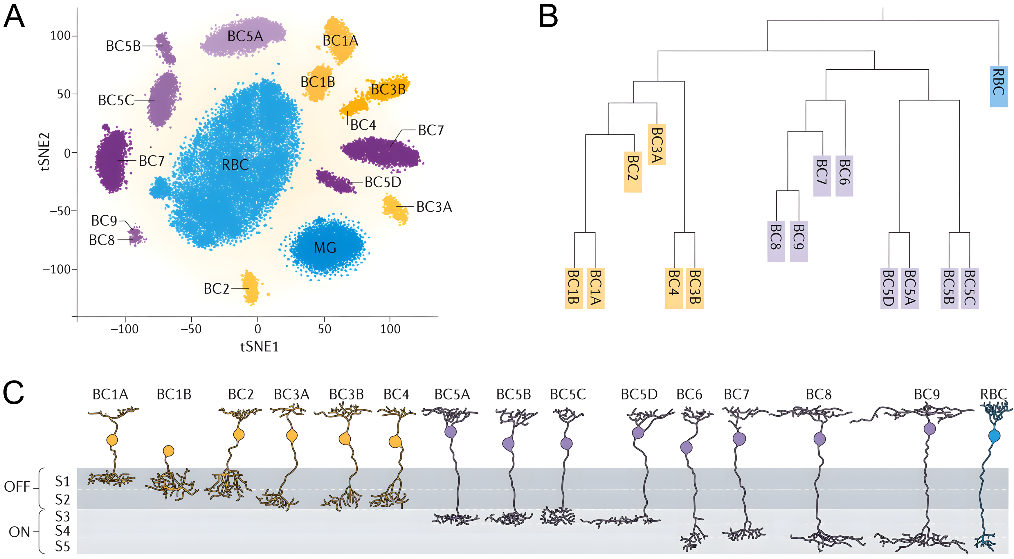
A. A t-SNE embedding plot showing clustering of ∼20,000 bipolar cells (BCs) that were isolated by fluorescence-activated cell sorting from a visual system homeobox 2 gene promoter-driven green fluorescent protein (GFP)-expressing (Vsx2-GFP) transgenic mouse line, in which GFP is expressed in all BCs and Muller glial (MG) cells and profiled by Drop-seq. The tSNE plot provides a convenient way to display cell clusters, as defined by a high-dimensional analysis of correlations in gene expression, in two dimensions.
B. Relationships among the BC types are shown in the form of a dendrogram that was created based on their transcriptomic similarity
Original figure from Zeng & Sanes (2017).
In conclusion, studying cell types, either clustered or part of a continuum, defined at least from morphological properties and at best from molecular, structural and functional features, is helpful to study neural function, because neural cell-types correlate with the features which themselves correlate with neural function: anatomy, connectivity, morphology and physiology.
Wrapping Up: Why Neuron Cell-Typing Matters
The classification of neurons isn’t just taxonomic busywork — it’s a practical framework that helps us make sense of the brain. Throughout this piece, I’ve outlined how classifying neurons provides a common nomenclature for reproducibility, enables molecular targeting techniques, establishes foundations for evolutionary and developmental studies, and most importantly, helps us understand neural function.
Cell typing approaches have evolved from Cajal’s purely morphological observations to formal machine learning frameworks that can work in high-dimensional feature spaces. These approaches can reveal both discrete clusters (as in retinal bipolar cells) and functional continua (as seen in some cortical populations), accommodating the full spectrum of neuronal diversity. Our recent paper (Beau et al., 2025) illustrates this point directly: a semi-supervised classifier can use spike waveforms, firing statistics, and anatomical location to reliably predict cell identity in the cerebellar cortex.
The connection between cell types and function isn’t arbitrary - it’s rooted in the biological relationships between a neuron’s molecular properties and its computational role. This relationship has been demonstrated in specific systems, such as striatal medium spiny neurons and retinal circuits. However, significant challenges remain in understanding how universally this pattern holds. It’s unclear how well these relationships generalize across different brain regions, particularly in areas where circuit ‘functions’ aren’t well defined. Furthermore, the robustness of cell typing to different feature spaces is an open question - what happens when neuronal properties exist along a continuum but their functions are discrete, or vice versa? As multimodal approaches to cell typing advance, a key challenge will be reconciling potential mismatches between structural classifications and functional roles across diverse neural systems.
In short, I care about neuron cell-typing because neurons that look alike probably work alike - and understanding these groupings gives us a much needed handle on the brain’s overwhelming complexity.
Bibliography
- . "A deep learning strategy to identify cell types across species from high-density extracellular recordings," Cell , 2025. doi: 10.1016/j.cell.2025.01.041
- . "The importance of Marr’s three levels of analysis for understanding cerebellar function," Computational Theories and their Implementation in the Brain: The legacy of David Marr 79 , 2016. doi: 10.1093/acprof:oso/9780198749783.003.0004
- . "Classes and continua of hippocampal CA1 inhibitory neurons revealed by single-cell transcriptomics," PLoS biology 16(6): e2006387 , 2018. doi: 10.1371/journal.pbio.2006387
- . "A transcriptomic atlas of mouse cerebellar cortex comprehensively defines cell types," Nature 598(7879): 214–219 , 2021. doi: 10.1038/s41586-021-03220-z
- . "A transcriptomic axis predicts state modulation of cortical interneurons," Nature 607(7918): 330–338 , 2022. doi: 10.1038/s41586-022-04915-7
- . "Neuronal cell-type classification: challenges, opportunities and the path forward," Nature Reviews Neuroscience 18(9): 530–546 , 2017. doi: 10.1038/nrn.2017.85